#specific packages for assumptions testing
library(car)             #used for several assumption checks
library(ggResidpanel)    #used for assumptions checks through plots
library(expss)           #used for frequency tables

#general packages
library(rio)             #loading data
library(tidyverse)       #data manipulation and plotting
library(broom)           #for asssumptions

#Data
ESS9NL <- import("data/ESS9e03, Netherlands.sav")13 Logistic Regression Assumptions
All models are built on simplifying assumptions. In this chapter, we’ll learn how to examine the assumptions underlying a logistic regression model:
- No excessive multicollinearity
- Linearity of the logit
- Limited impact of outliers and influential cases
Here are the packages that we will use and our data:
Of course, we need a model to examine. We will examine vote_model4 from last chapter, which predicts voter turnout based on age, gender, ideology, and trust in politicians. Here are the data preparation steps we took last time along with the model.
#Data Preparation
ESS9NL <- ESS9NL |>
#Factorize our IVs
mutate(gndr_F = factorize(gndr),
vote_F = factorize(vote)) |>
#Remove Not Eligible to Vote Category from vote
mutate(vote_F = na_if(vote_F,"Not eligible to vote")) |>
#Relevel our variables like we did last time
mutate(vote_F = relevel(vote_F, "No"),
gndr_F = relevel(gndr_F, "Female"))
#Subset of our data
ESS9NL_glm <- ESS9NL |>
filter(complete.cases(vote_F, gndr_F, agea, trstplt, lrscale))
#Our model
Vote_model4 <- glm(vote_F ~ gndr_F + agea + trstplt + lrscale,
data = ESS9NL_glm, family = "binomial")
#Check the output
summary(Vote_model4)- 1
- We subset the data in our last chapter so that we could compare multiple models against one another. Creating a dataset without missing observations on the variables in our model also makes it slightly easier to examine some of the assumptions below.
Call:
glm(formula = vote_F ~ gndr_F + agea + trstplt + lrscale, family = "binomial",
    data = ESS9NL_glm)

Coefficients:
             Estimate Std. Error z value Pr(>|z|)
(Intercept) -0.284194   0.380455  -0.747    0.455
gndr_FMale   0.043281   0.154201   0.281    0.779
agea         0.018349   0.004503   4.075 4.61e-05 ***
trstplt      0.195020   0.038706   5.039 4.69e-07 ***
lrscale      0.029257   0.039306   0.744    0.457
---
Signif. codes:  0 '***' 0.001 '**' 0.01 '*' 0.05 '.' 0.1 ' ' 1

(Dispersion parameter for binomial family taken to be 1)

    Null deviance: 1173.9  on 1424  degrees of freedom
Residual deviance: 1135.3  on 1420  degrees of freedom
AIC: 1145.3

Number of Fisher Scoring iterations: 4
13.1 No excessive multicollinearity
We can check for excessive multicollinearity using the vif() command from the car package, much as we did with linear regression models ( Section 7.2). The same interpretative rules of thumb are used here as well.
vif(Vote_model4) gndr_F agea trstplt lrscale
1.013505 1.018080 1.019284 1.013647 The statistics above indicate that we do not have a problem with excessive multicollinearity.
13.2 Linearity of the logit
Logistic regression models make the assumption that changes in the log of the odds (the logit) that Y = 1 are linear. We can examine this assumption using the augment() command from the broom package. This command will create a data object with the variables in our model as well as some important assumption-related statistics. Here is a preview:
augment(Vote_model4)# A tibble: 1,425 × 11
vote_F gndr_F agea trstplt lrscale .fitted .resid .hat .sigma .cooksd
<fct> <fct> <dbl> <dbl> <dbl> <dbl> <dbl> <dbl> <dbl> <dbl>
1 Yes Female 32 6 5 1.62 0.601 0.00238 0.894 0.0000947
2 No Male 57 7 5 2.32 -2.20 0.00175 0.893 0.00356
3 Yes Female 45 8 5 2.25 0.448 0.00220 0.894 0.0000467
4 Yes Female 34 7 5 1.85 0.540 0.00237 0.894 0.0000749
5 Yes Male 67 6 6 2.33 0.430 0.00188 0.894 0.0000365
6 No Female 85 5 4 2.37 -2.22 0.00330 0.893 0.00710
7 Yes Female 40 7 5 1.96 0.513 0.00199 0.894 0.0000561
8 Yes Male 71 8 7 2.83 0.339 0.00245 0.894 0.0000292
9 Yes Female 84 5 5 2.38 0.421 0.00310 0.894 0.0000577
10 Yes Male 24 7 5 1.71 0.576 0.00360 0.894 0.000131
# ℹ 1,415 more rows
# ℹ 1 more variable: .std.resid <dbl>
Output Explanation
votethroughlrscale: This is our raw data - the actual observed values for each respondent on our survey for the variables in our model. The names of these columns, and how many there are, would naturally be different in your examples..fitted: These are the “fitted’ or predicted values for each observation based on the model on a logit scale (i.e., these are not predicted probabilities but predicted log of the odds)..resid: Residual values from our model. More specifically, these are known as “deviance residuals”..hat: The diagonal of the hat matrix, which can be ignored..sigma: The estimated residual standard deviation when an observation is dropped, which can also be ignored..cooksd: Cook’s D values (see below)..std.resid: Standardized residuals (see below).
Later on we will want to investigate potential outliers and influential cases. We will thus work with the output of this command:
model4_augmented <- augment(Vote_model4, data = ESS9NL_glm)augment(Vote_model4, data=ESS9NL_glm)-
We have added
data = ESS9NL_glmto this version of the command. This creates an object with all of the columns above as well as all of the other variables in the dataset used to fit the model (ESS9NL_glm). This is useful for investigating potential outliers and influential cases in more detail. However, it requires that the dataset in question does not contain observations not in the model (i.e., observations with missing values on one or more of the variables in the model). This is why we subset ourESS9NLdataset in an earlier code chunk.
We assess the linearity of the logit assumption by plotting the data created by augment(). Specifically, we create a scatterplot with a loess line where the y-axis is the .fitted column (the predicted logit for each observation) and the x-axis is a continuous independent variable. We do this for each continuous variable in the model. Note: We do not need to do this for factor predictor variables.
# Age
ggplot(model4_augmented, aes(x = agea, y = .fitted)) +
  geom_point() +
  geom_smooth(method = "loess")
`geom_smooth()` using formula = 'y ~ x'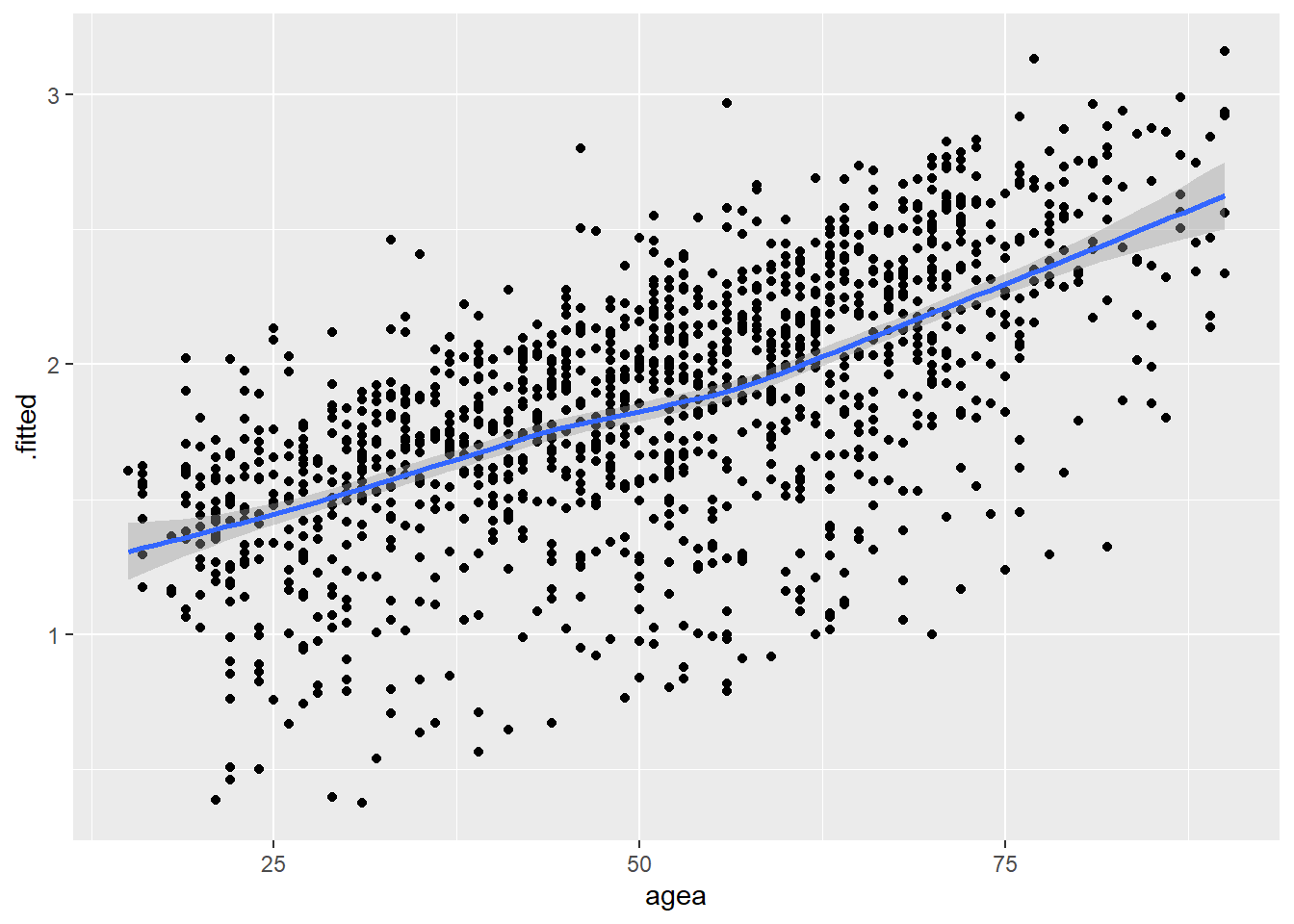
# Trust in Politicians
ggplot(model4_augmented, aes(x = trstplt, y = .fitted)) +
  geom_point() +
  geom_smooth(method = "loess")
`geom_smooth()` using formula = 'y ~ x'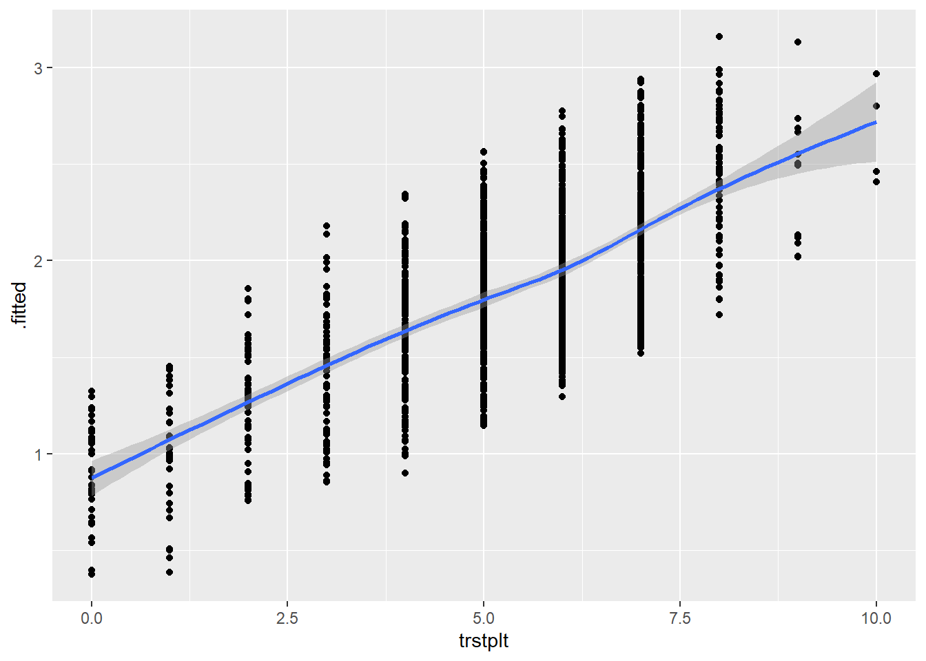
# LR Scale
ggplot(model4_augmented, aes(x = lrscale, y = .fitted)) +
  geom_point() +
  geom_smooth(method = "loess")
`geom_smooth()` using formula = 'y ~ x'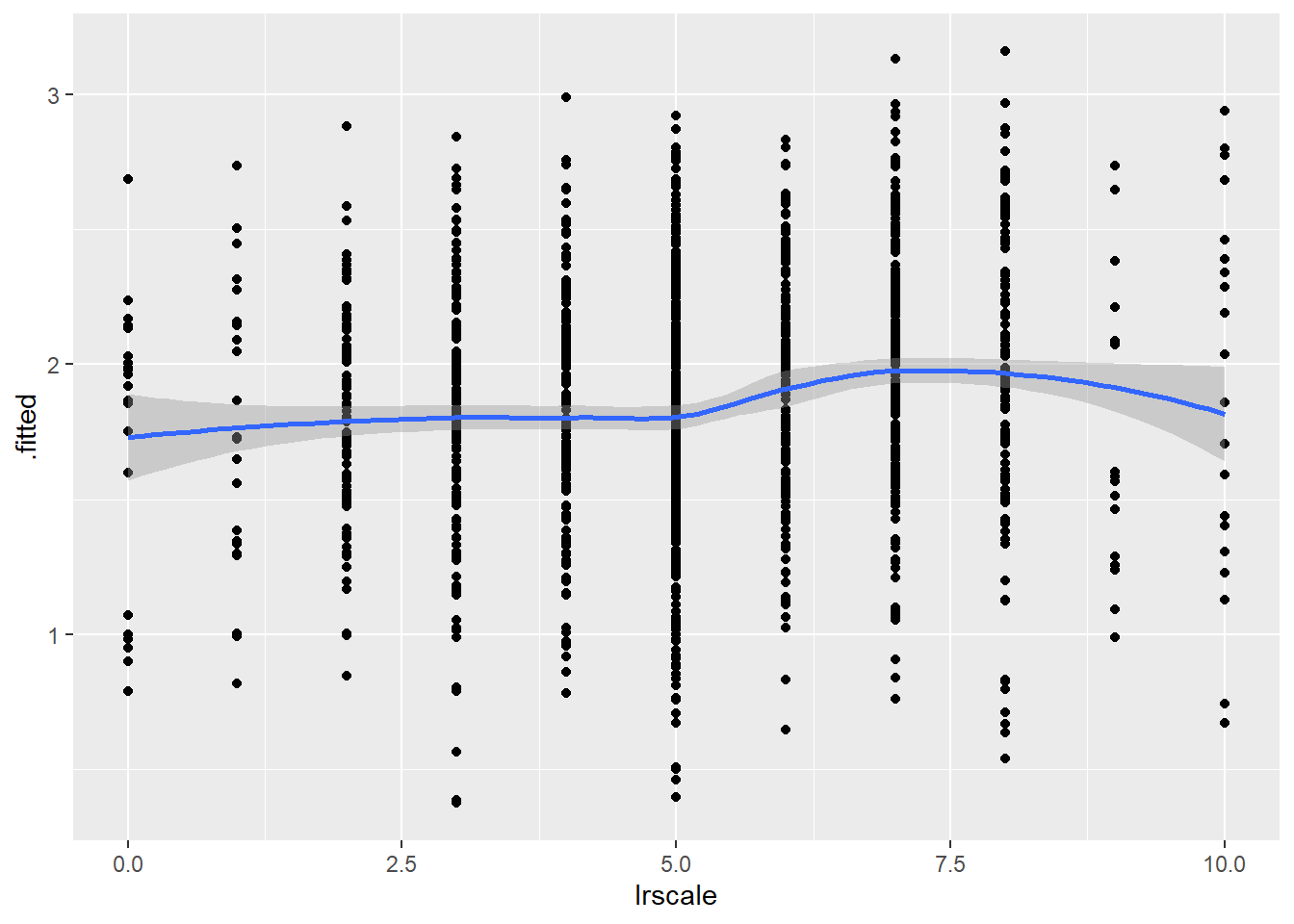
We are looking to see if the loess line shows a substantial deviation from linearity. There is no evidence of this in the figures above. We can thus say that this assumption is not violated.
13.3 Limited impact of outliers and influential cases
We used the augment() function above to create a data object that contains standardized residuals and Cook’s distance statistics for our observations as well as other variables from our original dataset that were not included in our model. We can use this data to investigate this assumption. We will first look at outliers and then at influential cases.
13.3.1 Outliers
We begin by looking at the summary statistics for the standardized residuals:
summary(model4_augmented$.std.resid) Min. 1st Qu. Median Mean 3rd Qu. Max.
-2.3983 0.4104 0.5040 0.1870 0.5916 1.0319 This output can help us understand whether there are any observations that cross the thresholds we use to assess this assumption (|1.96|, |2.58|, |3.29|), although it does not tell us how many might do so. Here, we do not observe any observations crossing either of the two highest thresholds (|2.58|, |3.29|). However, we do see at least one observation with an absolute value greater than 1.96 (the minimum value of the standardized residual is -2.398).
We can assess how many observations cross this threshold by creating a dummy variable (0 = .std.resid < |1.96|, 1 = .std.resid > |1.96|) and inspecting a frequency table.1 Here is an example of how to do so - see Section 7.6.1 for syntax relating to the threshold values of 2.58 and 3.29.
#Create the dummy variable:
model4_augmented <- model4_augmented |>
  mutate(SRE1.96 = case_when(
    .std.resid > 1.96 | .std.resid < -1.96  ~ 1,
    .std.resid > -1.96 & .std.resid < 1.96 ~ 0
  ))

#What percentage crosses the threshold?
fre(model4_augmented$SRE1.96)| model4_augmented$SRE1.96 | Count | Valid percent | Percent | Responses, % | Cumulative responses, % |
|---|---|---|---|---|---|
| 0 | 1344 | 94.3 | 94.3 | 94.3 | 94.3 |
| 1 | 81 | 5.7 | 5.7 | 5.7 | 100.0 |
| #Total | 1425 | 100 | 100 | 100 | |
| <NA> | 0 | 0.0 |
5.7% of observations have a standardized residual greater than |1.96|. We could examine whether these observations are substantially impacting the parameters of our model by re-running the model and subsetting the data to only include observations with a value of 0 on the dummy variable we just created (SRE1.96). For instance:
Vote_model41.96 <- glm(vote_F ~ gndr_F + agea + trstplt + lrscale,
                       data = subset(model4_augmented, SRE1.96 == 0),
                       family = "binomial")
13.3.2 Influential cases
We examine the Cook’s D values in our augmented dataset in order to investigate whether there are any concerning influential cases.
First, we can look at the summary of the Cook’s D values; see Section Section 7.6.2 for the rules of thumb we use when assessing these values. Second, we can visually inspect these values using the resid_panel() command from the ggResidpanel.
#Summary of the Cook's D values
summary(model4_augmented$.cooksd)
Min. 1st Qu. Median Mean 3rd Qu. Max.
2.331e-05 5.117e-05 8.959e-05 7.085e-04 2.442e-04 1.668e-02 #Plot
resid_panel(Vote_model4, plots = c("cookd"))Warning in helper_plotly_label(model): NAs introduced by coercion
Warning in helper_plotly_label(model): NAs introduced by coercion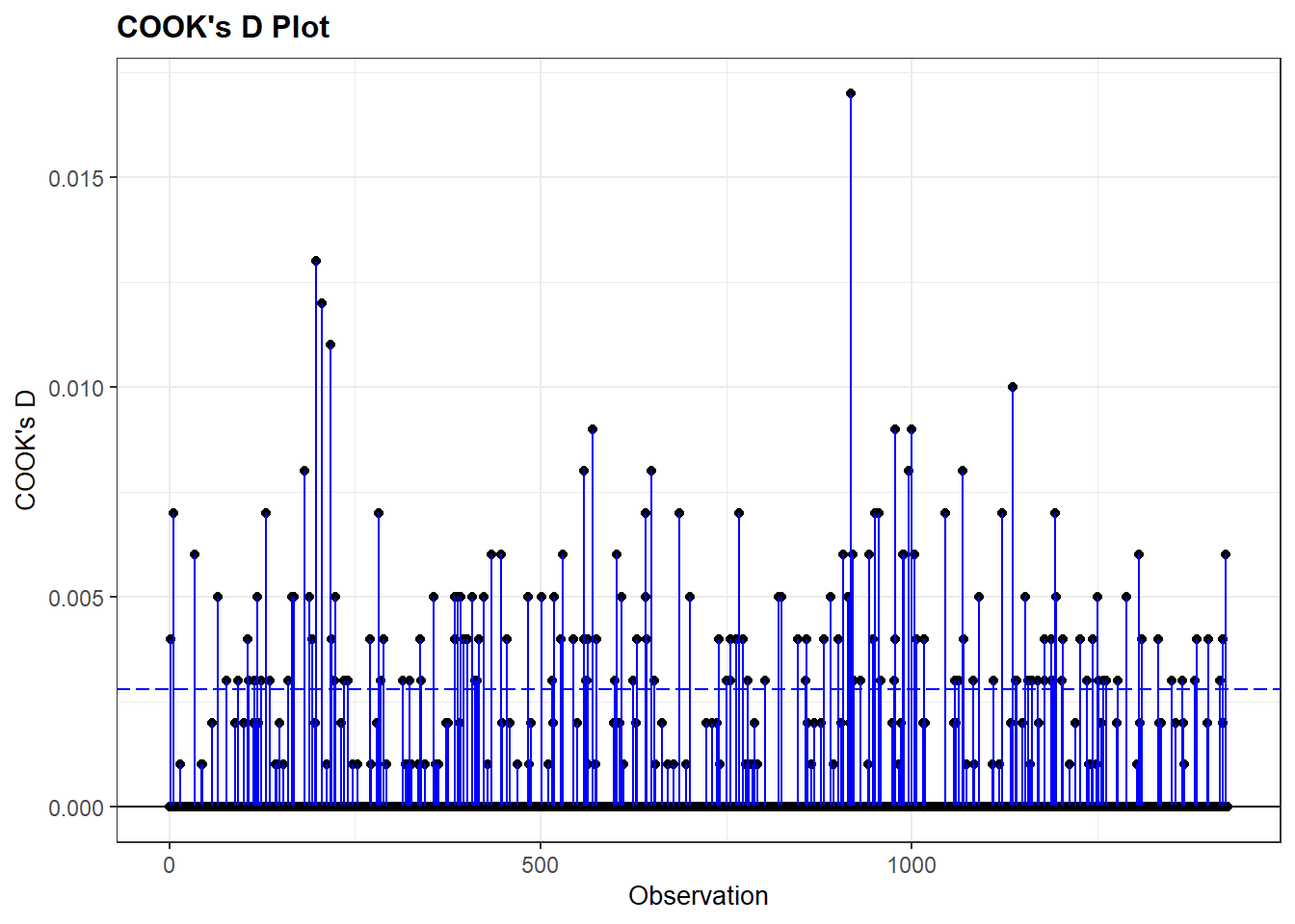
The Cook’s D values are very small with a maximum value of around 0.017. There is little evidence that we have a problem here. If we did find higher values, then we could further examine them by, for instance, re-running our model with them filtered out. We could also examine the influential cases themselves to see if there is an explanation for why they are so influential.
Calculating the mean of this 0/1 variable would accomplish the same end.↩︎