#Packages
library(sjPlot)            #Dataset overviews
library(modelsummary)      #Regression & correlation tables
library(broom)             #Model summaries, including coefficients
library(rio)               #Importing data
library(tidyverse)         #Data management & plotting

#Data
anes <- import("data/anes_interactions.rda")15 Including an Interaction Term in a Regression Model
Thus far we have been investigating statistical models wherein we predict a dependent variable with one or more independent variables. One goal of these models has been to identify the relationship between a predictor variable and the dependent variable that is ‘independent’ of the influence of the other predictors. For instance, what is the relationship between a person’s party affiliation and their evaluation of specific politicians, such as a country’s Prime Minister or President, when holding the effects of other characteristics of the individual “constant”?
Researchers do not always want to hold another predictor in the model “constant” in this way. Instead, they may want to know if two independent variables have an interactive relationship when predicting the dependent variable. For instance, we might ask whether the relationship between partisanship and evaluations of a major political leader is exactly the same among people who think things are going well in the country and those that think things are going poorly. Examining this type of question requires us to add an interaction term to our model. This chapter shows you how to do just that with a focus on both linear and logistic regression models.
Here are the packages that we will use in this chapter as well as our data:
The dataset that we will use in this chapter, and the ones to come, contains survey data selected from the 2020 American National Election Studies or ANES for short. The 2020 ANES was conducted right around the time of the 2020 Presidential elections featuring a contest between then President Donald Trump (Republican Party) and his challenger Joseph Biden (Democratic Party). This dataset has already been “cleaned”: missing value codes have been converted to “NA” and binary/categorical variables have been converted into factor variables. Let’s take a look at its contents:
view_df(anes)| ID | Name | Label | Values | Value Labels |
| 1 | trump | Evaluation of Donald Trump | range: 0-100 | |
| 2 | biden | Evaluation of Joe Biden | range: 0-100 | |
| 3 | socialists | Evaluation of Socialists | range: 0-100 | |
| 4 | right_track | Is Country Heading in Right Direction or the Wrong Track |
Wrong Track Right Direction |
|
| 5 | vote2016 | Vote Choice in 2016 Pres Election | Clinton Vote Trump Vote |
|
| 6 | pid | Party Identification | 1 2 3 4 5 6 7 |
Strong Democrat Not Strong Democrat Lean Democrat Independent Lean Republican Not Strong Republican Strong Republican |
| 7 | age | Age in years | range: 18-80 | |
| 8 | rural_urban | Type of Area Respondent Lives In | Suburb Rural Small Town City |
|
15.1 Adding an Interaction Term to a Regression Model
We can add multiple predictor variables to both a linear (lm) and logistic (glm) regression model using the ‘+’ sign. We can include an interaction between two predictor variables by using the ‘*’ sign instead.
For example, in this linear regression model we predict how respondents evaluated then candidate Joe Biden on a scale ranging from 0 (‘very cold or unfavorable’) to 100 (‘very warm or favorable’) using three predictor variables: (1) pid (the respondent’s partisan identity, which is a continuous variable ranging from 1 [“Strong Democrat”] to 7 [“Strong Republican”]); (2) right_track (a binary factor variable where 0 indicates the respondent thinks the “country is on the wrong track” and 1 that the “country is heading in the right direction”); (3) and rural_urban (a categorical variable concerning where the respondent lives with “suburb” as the reference category).
#Run the model and store results
biden_model <- lm(biden ~ pid + right_track + rural_urban, data = anes)

#Summary of results
summary(biden_model)
Call:
lm(formula = biden ~ pid + right_track + rural_urban, data = anes)

Residuals:
    Min      1Q  Median      3Q     Max
-83.656 -13.349   0.771  16.344  90.722

Coefficients:
                           Estimate Std. Error t value Pr(>|t|)
(Intercept)                 93.9170     0.6543 143.537  < 2e-16 ***
pid                        -10.2606     0.1364 -75.245  < 2e-16 ***
right_trackRight Direction -12.8153     0.6993 -18.326  < 2e-16 ***
rural_urbanRural            -4.1666     0.8219  -5.070 4.09e-07 ***
rural_urbanSmall Town       -2.9846     0.7011  -4.257 2.10e-05 ***
rural_urbanCity             -0.3076     0.6713  -0.458    0.647
---
Signif. codes:  0 '***' 0.001 '**' 0.01 '*' 0.05 '.' 0.1 ' ' 1

Residual standard error: 21.88 on 7141 degrees of freedom
  (1133 observations deleted due to missingness)
Multiple R-squared:  0.602, Adjusted R-squared:  0.6018
F-statistic:  2161 on 5 and 7141 DF,  p-value: < 2.2e-16
Evaluations of Biden become more negative on average as the pid measure increases in value, that is, as we move from the Democratic end of the scale to the Republican end of the scale. Respondents who state that the country is heading in the “right direction”, meanwhile, evaluate Biden worse on average than those who say that the country is “on the wrong track”. This is because answers to the right_track question reflect one’s impressions of the performance of then President Donald Trump: people saying ‘right direction’ had positive evaluations of Trump and, conversely, negatively ones of his opponent Biden.1
Perhaps we have some theory-driven reason to expect the relationship between partisanship and evaluations of Biden to vary based on whether people think things in the country are going well or not. Or, vice versa, we might have some reason to think that the effect of evaluations regarding how things were going in the country on evaluations of Biden depends on the person’s partisanship. We can examine these types of questions by adding an interaction between the two variables (pid and right_track) by using an asterisk (‘*’) rather than a plus sign (‘+’) to separate the two variables:
#Run the model and store results
biden_int <- lm(biden ~ pid * right_track + rural_urban, data = anes)

#Summary of results
summary(biden_int)
Call:
lm(formula = biden ~ pid * right_track + rural_urban, data = anes)

Residuals:
    Min      1Q  Median      3Q     Max
-84.834 -13.186   0.166  15.166  87.299

Coefficients:
                               Estimate Std. Error t value Pr(>|t|)
(Intercept)                     95.6585     0.6730 142.146  < 2e-16 ***
pid                            -10.8243     0.1468 -73.744  < 2e-16 ***
right_trackRight Direction     -33.1885     2.1600 -15.365  < 2e-16 ***
rural_urbanRural                -4.0838     0.8163  -5.003 5.79e-07 ***
rural_urbanSmall Town           -2.8082     0.6965  -4.032 5.60e-05 ***
rural_urbanCity                 -0.3202     0.6667  -0.480    0.631
pid:right_trackRight Direction   3.7144     0.3729   9.961  < 2e-16 ***
---
Signif. codes:  0 '***' 0.001 '**' 0.01 '*' 0.05 '.' 0.1 ' ' 1

Residual standard error: 21.73 on 7140 degrees of freedom
  (1133 observations deleted due to missingness)
Multiple R-squared:  0.6075,    Adjusted R-squared:  0.6072
F-statistic:  1842 on 6 and 7140 DF,  p-value: < 2.2e-16
Output Explanation
The structure of our output is the same as with our previous examples. However, we can see that there is now an extra term in the Coefficients box: “pid:right_trackRight Direction”.
When we separate two variables by an ‘*’, R will include both variables plus an interaction term multiplying the two variables with one another in the model. The name provided to the interaction term will be the names of the two variables separated by a colon as in the example above (“pid:right_trackRight Direction”).
Including an interaction term follows the same principles when using a logistic model. We demonstrate that here by predicting whether the person says the US is heading in the “right direction” (1) or not (0) (right_track). We use the following predictor variables: (1) vote2016, which records who the respondent reported voting for in the 2016 Presidential election (Hillary Clinton = 0, Donald Trump = 1; vote2016); age in years (age); and place of residence (rural_urban). We add an interaction between vote2016 and age in this example:
#Run the model and store results
righttrack_int <- glm(right_track ~ vote2016 * age + rural_urban,
                      family = "binomial", data = anes)

#Summary of results
summary(righttrack_int)
Call:
glm(formula = right_track ~ vote2016 * age + rural_urban, family = "binomial",
    data = anes)

Coefficients:
                        Estimate Std. Error z value Pr(>|z|)
(Intercept)            -2.952141   0.344679  -8.565  < 2e-16 ***
vote2016Trump Vote      2.820292   0.373350   7.554 4.22e-14 ***
age                    -0.009465   0.006296  -1.503   0.1328
rural_urbanRural        0.208129   0.111289   1.870   0.0615 .
rural_urbanSmall Town   0.110962   0.101173   1.097   0.2727
rural_urbanCity         0.160473   0.110704   1.450   0.1472
vote2016Trump Vote:age  0.012914   0.006823   1.893   0.0584 .
---
Signif. codes:  0 '***' 0.001 '**' 0.01 '*' 0.05 '.' 0.1 ' ' 1

(Dispersion parameter for binomial family taken to be 1)

    Null deviance: 5929.4  on 5132  degrees of freedom
Residual deviance: 4033.5  on 5126  degrees of freedom
  (3147 observations deleted due to missingness)
AIC: 4047.5

Number of Fisher Scoring iterations: 6
Interpretation
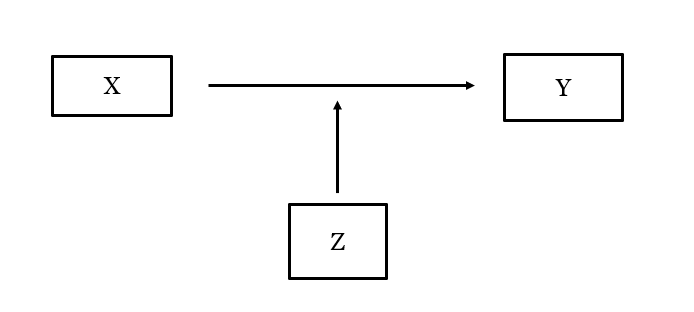
When estimating an interaction term, we are basically asking ourselves whether the relationship between a certain predictor (X) and the dependent variable (Y) is different when a second predictor (Z) takes on different values. The coefficient for the interaction term provides us with information about whether this is the case.
In our linear biden_int model, for instance, the interaction term is statistically significant: the relationship between pid and Biden evaluations may be different depending on whether the person says the country is on the wrong track or heading in the “right direction”.2 The interaction term in the logistic righttrack_int model, meanwhile, is not statistically significant using conventional standards of significance, which implies that the relationship between, for instance, age and beliefs about the country is the same regardless of whether we consider Clinton or Trump voters.
The coefficients for the variables being interacted with one another can be tricky to directly interpret. As a result, we will use R to calculate other statistical estimates to better understand the interaction effect:
- The marginal effect of one variable in the interaction at different values of the other variable in the interaction ( Chapter 16).
- The predicted values for specific value combination of the two variables in the interaction. ( Chapter 17)
15.2 Regression Tables
Our next two chapters will focus on communicating the results of regression models that feature interaction terms via plots. Here we will briefly note show how to present these results as a regression table using the modelsummary() function from the modelsummary library. The basic principles are the same as discussed in prior chapters (linear regression tables: Section 8.5 ; logistic regression tables: Section 14.2 ).
We will provide the results of our first two models in this example. We will show both the original model and the one that adds the interaction term side by side so that readers can see how our results change the interaction is added to the model.
# List of models
interaction_lm_models <- list(
biden_model, biden_int
)
#Create the table
modelsummary(interaction_lm_models,
stars = T,
coef_rename = c(
"(Intercept)" = "Intercept",
"pid" = "Party Identification",
"right_trackRight Direction" = "Country Heading in Right Direction?",
"rural_urbanRural" = "Rural Resident",
"rural_urbanSmall Town" = "Small Town Resident",
"rural_urbanCity" = "City Resident",
"pid:right_trackRight Direction" = "PID x Right Direction"),
gof_map = c("nobs", "r.squared", "adj.r.squared"),
title = "Predicting Biden Evaluations",
notes = "OLS coefficients with standard errors in parentheses; Reference category for place of residence = Suburbs.")- 1
- We first create a new “list” object containing the models we want to include in the table
- 2
- The name of the list object we just created
- 3
- This adds “stars” to signal statistical significance
- 4
-
We rename our variables for better communication via
coef_rename() - 5
-
We select which model fit statistics via
gof_map() - 6
-
We can give a title to the table via
title = - 7
-
And, finally, provide some notes at the bottom of the table via
notes =
| (1) | (2) | |
|---|---|---|
| + p < 0.1, * p < 0.05, ** p < 0.01, *** p < 0.001 | ||
| OLS coefficients with standard errors in parentheses; Reference category for place of residence = Suburbs. | ||
| Intercept | 93.917*** | 95.659*** |
| (0.654) | (0.673) | |
| Party Identification | -10.261*** | -10.824*** |
| (0.136) | (0.147) | |
| Country Heading in Right Direction? | -12.815*** | -33.188*** |
| (0.699) | (2.160) | |
| Rural Resident | -4.167*** | -4.084*** |
| (0.822) | (0.816) | |
| Small Town Resident | -2.985*** | -2.808*** |
| (0.701) | (0.697) | |
| City Resident | -0.308 | -0.320 |
| (0.671) | (0.667) | |
| PID x Right Direction | 3.714*** | |
| (0.373) | ||
| Num.Obs. | 7147 | 7147 |
| R2 | 0.602 | 0.607 |
| R2 Adj. | 0.602 | 0.607 |
The main thing we might want to change about a table like this is to change the placement of the interaction term coefficient. The default behavior is to place it at the bottom of the table. That is perfectly fine, but we might want to place it alongside the other variables within the interaction so that consumers of our table can consider these coefficients all at once. We can do this by changing coef_rename to coef_map in our syntax and moving the entry for the interaction term to where we want it to show up in the resulting table:
modelsummary(interaction_lm_models,
stars = T,
coef_map = c(
"(Intercept)" = "Intercept",
"pid" = "Party Identification",
"right_trackRight Direction" = "Country Heading in Right Direction?",
"pid:right_trackRight Direction" = "PID x Right Direction",
"rural_urbanRural" = "Rural Resident",
"rural_urbanSmall Town" = "Small Town Resident",
"rural_urbanCity" = "City Resident"),
gof_map = c("nobs", "r.squared", "adj.r.squared"),
title = "Predicting Biden Evaluations",
notes = "OLS coefficients with standard errors in parentheses; Reference category for place of residence = Suburbs.") - 1
-
We changed
coef_renametocoef_map - 2
-
We moved the part where we rename the interaction up and placed it after the second term in our interaction. This changes the order in which the coefficients are displayed in our table due to the use of
coef_map
| (1) | (2) | |
|---|---|---|
| + p < 0.1, * p < 0.05, ** p < 0.01, *** p < 0.001 | ||
| OLS coefficients with standard errors in parentheses; Reference category for place of residence = Suburbs. | ||
| Intercept | 93.917*** | 95.659*** |
| (0.654) | (0.673) | |
| Party Identification | -10.261*** | -10.824*** |
| (0.136) | (0.147) | |
| Country Heading in Right Direction? | -12.815*** | -33.188*** |
| (0.699) | (2.160) | |
| PID x Right Direction | 3.714*** | |
| (0.373) | ||
| Rural Resident | -4.167*** | -4.084*** |
| (0.822) | (0.816) | |
| Small Town Resident | -2.985*** | -2.808*** |
| (0.701) | (0.697) | |
| City Resident | -0.308 | -0.320 |
| (0.671) | (0.667) | |
| Num.Obs. | 7147 | 7147 |
| R2 | 0.602 | 0.607 |
| R2 Adj. | 0.602 | 0.607 |
Here, we have moved the interaction term up in the table so that it comes right after the two other variables in the interaction (pid and right_track).
Warning!
We can use coef_map to alter the order of coefficients in our table as above. This is not usually needed but can be handy in some circumstances. But, do note that coef_map is type sensitive and will only show coefficients when you have correctly written out their underlying name. Here is an example, for instance, where we make two mistakes: we write “right_trackRight direction” rather than the correct “right_trackRight Direction” and we write “rural_urbancity” instead of “rural_urbanCity”:
modelsummary(interaction_lm_models,
stars = T,
coef_map = c(
"(Intercept)" = "Intercept",
"pid" = "Party Identification",
"right_trackRight direction" = "Country Heading in Right Direction?",
"pid:right_trackRight Direction" = "PID x Right Direction",
"rural_urbanRural" = "Rural Resident",
"rural_urbanSmall Town" = "Small Town Resident",
"rural_urbancity" = "City Resident"),
gof_map = c("nobs", "r.squared", "adj.r.squared"),
title = "Predicting Biden Evaluations",
notes = "OLS coefficients with standard errors in parentheses") - 1
- We changed “Direction” to “direction”
- 2
- We changed “City” to “city”
| (1) | (2) | |
|---|---|---|
| + p < 0.1, * p < 0.05, ** p < 0.01, *** p < 0.001 | ||
| OLS coefficients with standard errors in parentheses | ||
| Intercept | 93.917*** | 95.659*** |
| (0.654) | (0.673) | |
| Party Identification | -10.261*** | -10.824*** |
| (0.136) | (0.147) | |
| PID x Right Direction | 3.714*** | |
| (0.373) | ||
| Rural Resident | -4.167*** | -4.084*** |
| (0.822) | (0.816) | |
| Small Town Resident | -2.985*** | -2.808*** |
| (0.701) | (0.697) | |
| Num.Obs. | 7147 | 7147 |
| R2 | 0.602 | 0.607 |
| R2 Adj. | 0.602 | 0.607 |
Oh no! We no longer see coefficients for the two variables that we mis-spelled in our syntax.
The warning here is that if you do use coef_map in this way in your future work, then double check your spellings and your output lest you mistakenly leave something quite critical out of your table. You can learn more about the coef_map option at the modelsummary website (link)
Our dataset also has a measure of evaluations of Donald Trump (the variable named
trump). The average evaluation of Trump among those saying the country was heading in the “right direction” was 83.2 on this 0-100pt scale, while it was 25.4 among those saying things were heading down the “wrong track”.↩︎But note that interaction terms are “symmetrical”. We can also talk about whether the difference in Biden evaluations based on saying “right direction” or “wrong track” is the same for Strong Democrats (pid = 1) as for Not Strong Democrats (pid = 2) and so on. When we interpret an interaction model we must first discern what variable is supposed to be the “X” variable and which is supposed to be the “Z” (or moderator) variable as this effects how we use the model”s results.↩︎