12.1.1 Confidence interval for a single proportion
12.1.1.1 Calculating ‘by hand’ using R
One approach is to calculate the normal approximation of the binomial distribution (Wald interval), as described in the OpenIntro book. This is basically the same as doing the ‘manual’ calculation, but in R.
As an example, we use a survey of voters in which 23% indicate to support the Conservatives. We estimate a 95% confidence interval for this estimate:
# Define input (change these you appropriate values)p_hat =0.23n =1000confidence =0.95# Perform calculations (no need to change anything here)se =sqrt(p_hat * (1- p_hat)/ n) # Calculate SEz_star =qnorm((1+ confidence) /2) # Calculate z*-value lower = p_hat - z_star * se # Lower bound CIupper = p_hat + z_star * se # Upper bound CIc(lower, upper)
[1] 0.203917 0.256083
12.1.1.2 Using summary data
When you have only summary data, i.e. information about the sample size and sample proportion, we recommend using prop.test for calculating a confidence interval for a single proportion.[^3] The function prop.test is part of the package stats, which is one of the few packages that R automatically loads when it starts.
# Define inputp_hat =0.23n =1000# Run the actual testprop.test(x = p_hat * n, n = n, conf.level =0.95)
    1-sample proportions test with continuity correction

data:  p_hat * n out of n, null probability 0.5
X-squared = 290.52, df = 1, p-value < 2.2e-16
alternative hypothesis: true p is not equal to 0.5
95 percent confidence interval:
 0.2045014 0.2576046
sample estimates:
   p
0.23
Note: The results from the calculation by hand and from the function prop.test are slightly different. This is due to the fact that prop.test uses a slightly more complicated formula for calculating the confidence interval (Wilson score interval), also incorporating a ‘continutiy correction’ (which accounts for the fact that we are using a continuous normal distribution to approximate a discrete phenomenon, i.e. the number of successes).
prop.test
This is the function that conducts a test for a proportion and its confidence interval.
x = p_hat * n
The first value specified should be the number of successes. In our example his is the number of people supporting the Conservatives. We can calculate this as the sample proportion (\(\hat{p}\)) times the sample size.
n = n
The second value specified should be the number of trials (read: the number of observations in our dataset). In our case: the number of respondents in the dataset.
conf.level = 0.95
This determines the confidence level. The default is 0.95 which corresponds to a 95% confidence interval.
12.1.1.3 Variables in a data frame
If you have a data frame with a variable that represents successes (or not) for each case, we can use the following procedure. In our example we have a variable that records the vote intention of a respondent, which is either Conservative or Other party:
# For this example, we create a dataset of 1000 respondents with 230 expressing support for the Conservativesexample_data =data.frame(party_choice =factor(c(rep("Conservatives", 230), rep("Other party", 770))))table(example_data$party_choice)
Conservatives   Other party
          230           770
If we have data like this, we can directly calculate the confidence interval by running prop.test for the table:
The first argument is a table of our variable of interest, which we can create by this code. If you use your own data, replace example_data with the name of your data frame and party_choice with the name of the variable of interest.1
Note: The table should include only two categories. R will calculate the confidence interval for the first category in the table (in our case: Conservatives).2
conf.level = 0.95
This determines the confidence level. The default is 0.95 which corresponds to a 95% confidence interval.
    1-sample proportions test with continuity correction

data:  table(example_data$party_choice), null probability 0.5
X-squared = 290.52, df = 1, p-value < 2.2e-16
alternative hypothesis: true p is not equal to 0.5
95 percent confidence interval:
 0.2045014 0.2576046
sample estimates:
   p
0.23
12.1.2 Hypothesis tests for a single proportion
12.1.2.1 Summary data
When you only have information about the sample size and the proportion, we recommend using prop.test for conducting a hypothesis test.3
# Define inputp_hat =0.23n =1000# Run the actual testprop.test(x = p_hat * n, n = n, p =0.25,alternative ="two.sided")
    1-sample proportions test with continuity correction

data:  p_hat * n out of n, null probability 0.25
X-squared = 2.028, df = 1, p-value = 0.1544
alternative hypothesis: true p is not equal to 0.25
95 percent confidence interval:
 0.2045014 0.2576046
sample estimates:
   p
0.23
prop.test
This is the function that conducts a test for a proportion.
x = p_hat * n
The first value specified should be the number of successes. We can calculate this as the sample proportion (\(\hat{p}\)) times the sample size.
n = n
The second value specified should be the number of trials (read: the number of observations in our dataset). In our case: the number of respondents in the dataset.
p = 0.25
This specifies the hypothesized null value. In this example this is 0.25 or 25%, so we are testing the null hypothesis \(\mu_0 = 0.25\)
alternative = "two.sided"
Determine whether we want to use a two sided-test, or a one-sided test. Options are “two.sided” (default), “less” (when \(H_1: \mu < p\)) or “greater” (when \(H_1: \mu > p\)).
12.1.2.2 Variables in a data frame
If you have a data frame with a variable that represents successes (or not) for each case, we can input this data directly into prop.test. In our example we have a variable that records the vote intention of a respondent, which is either Conservative or Other party (for the preparation of the data see [Single proportion confidence intervals for variables in a data frame]).
The first argument is a table of our variable of interest, which we can create by this code. If you use your own data, replace example_data with the name of your data frame and party_choice with the name of the variable of interest.
Note: The table should include only two categories. R will perform the test that the proportion for the first category is equal to the hypothesized value (p, see below).
p = 0.25
This specifies the hypothesized null value. In this example this is 0.25 or 25%, so we are testing the null hypothesis \(\mu_0 = 0.25\)
alternative = "two.sided"
Determine whether we want to use a two sided-test, or a one-sided test. Options are “two.sided” (default), “less” (when \(H_1: \mu < p\)) or “greater” (when \(H_1: \mu > p\)).
    1-sample proportions test with continuity correction

data:  table(example_data$party_choice), null probability 0.25
X-squared = 2.028, df = 1, p-value = 0.1544
alternative hypothesis: true p is not equal to 0.25
95 percent confidence interval:
 0.2045014 0.2576046
sample estimates:
   p
0.23
12.2 Reporting the results from a hypothesis test for a single proportion
#Obtain z-value based on manual calculation# Define inputp_hat =0.12n =1500p =0.10z <- (p_hat-p)/(sqrt((p*(1-p)/n)))z
[1] 2.581989
2*pnorm(q=z, lower.tail=FALSE)
[1] 0.009823275
# Run the actual testprop.test(x = p_hat * n, n = n, p =0.10,alternative ="two.sided",correct =FALSE)
    1-sample proportions test without continuity correction

data:  p_hat * n out of n, null probability 0.1
X-squared = 6.6667, df = 1, p-value = 0.009823
alternative hypothesis: true p is not equal to 0.1
95 percent confidence interval:
 0.1045180 0.1374233
sample estimates:
   p
0.12
Output explanation
the probability of finding the observed (\(z\) or \(\chi^2\), given the null hypothesis (p-value) is given as follows:
in R, see p-value = 0.009823. Note: If the value is very close to zero, R may use the scientific notation for small numbers (e.g. 2.2e-16 is the scientific notation of 0.00000000000000022). In these cases, write p < 0.001 in your report.
12.2.0.1 Reporting
If you calculate the results by hand and obtain a z-score, then the correct report includes:
A conclusion about the null hypothesis; followed by
Information about the sample percentage and the population percentage.
\(z\) = the value of z.
p = p-value. When working with statistical software, you should report the exact p-value that is displayed.
in R, small values may be displayed using the scientific notation (e.g. 2.2e-16 is the scientific notation of 0.00000000000000022.) This means that the value is very close to zero. R uses this notation automatically for very small numbers. In these cases, write p < 0.001 in your report.
If you calculate the results using prop.test and obtain a \(\chi^2\)-score, then the correct report includes:
A conclusion about the null hypothesis; followed by
Information about the sample percentage and the population percentage.
\(\chi^2\) = the value of chi-square, followed by the degrees of freedom in brackets.
p = p-value. When working with statistical software, you should report the exact p-value that is displayed.
in R, small values may be displayed using the scientific notation (e.g. 2.2e-16 is the scientific notation of 0.00000000000000022.) This means that the value is very close to zero. R uses this notation automatically for very small numbers. In these cases, write p < 0.001 in your report.
Report
✓ The percentage of supporters found in our sample (N = 1500) who support the Socialist Party (12%) is statistically significantly different from the percentage of the entire population (10%), z=2.58, p=0.1394.
✓ The percentage of supporters found in our sample (N = 1500) who support the Socialist Party (12%) is statistically significantly different from the percentage of the entire population (10%), \(\chi^2\) (1)=6.6667, p=0.0098.
12.3 Comparing two proportions
Last week, we calculated a confidence interval for a single proportion. This week we cover two (independent) proportions. The calculations below apply to the case where the two proportions are drawn from different samples or subsamples, for example the support for a party in two separate opinion polls or the left-right position of respondents who live in the capital city and those who do not live there (these groups are independent because you can only belong to one).
12.3.1 Confidence interval for the difference between two proportions
We use the CPR data set from the openintro package (see p. 218). The data set contains data on patients who were randomly divided into a treatment group where they received a blood thinner or the control group where they did not receive a blood thinner. The outcome variable of interest was whether the patients survived for at least 24 hours.
library(tidyverse)
── Attaching core tidyverse packages ──────────────────────── tidyverse 2.0.0 ──
✔ dplyr     1.1.4     ✔ readr     2.1.5
✔ forcats   1.0.0     ✔ stringr   1.5.1
✔ ggplot2   3.5.2     ✔ tibble    3.2.1
✔ lubridate 1.9.4     ✔ tidyr     1.3.1
✔ purrr     1.0.2
── Conflicts ────────────────────────────────────────── tidyverse_conflicts() ──
✖ dplyr::filter() masks stats::filter()
✖ dplyr::lag()    masks stats::lag()
ℹ Use the conflicted package (<http://conflicted.r-lib.org/>) to force all conflicts to become errors
library(openintro)
Warning: package 'openintro' was built under R version 4.4.3
Loading required package: airports
Warning: package 'airports' was built under R version 4.4.3
Loading required package: cherryblossom
Warning: package 'cherryblossom' was built under R version 4.4.3
Loading required package: usdata
Warning: package 'usdata' was built under R version 4.4.3
library(flextable)
Attaching package: 'flextable'

The following object is masked from 'package:purrr':

    compose
data(cpr)# Refactor variables to ensure the order is the same as in the textbook tablecpr <- cpr |>mutate(group =factor(group, levels =c("control", "treatment"), ordered =TRUE),outcome =factor(outcome, levels =c("survived", "died"), ordered =TRUE))table_example <-proc_freq(x = cpr, row ="group", col ="outcome", include.row_percent =FALSE, include.column_percent =FALSE, include.table_percent =FALSE) table_example
group
outcome
survived
died
Total
control
11
39
50
treatment
14
26
40
Total
25
65
90
Note that we usually put the independent variable in the columns. However, the book does not follow this convention.
12.3.1.1 Calculating ‘by hand’ using R
To calculate a 90 % confidence interval of the difference for the survival rates (\(p_{1}\) and \(p_{2}\)) by hand, we can write:
# Define input (change these according to your values)p_hat_1 =14/40# Treatment groupp_hat_2 =11/50# Control groupn_1 =40n_2 =50confidence =0.9# Perform calculations (no need to change anything here)p_hat = p_hat_1 - p_hat_2se =sqrt((p_hat_1*(1-p_hat_1)/n_1) + (p_hat_2*(1-p_hat_2)/n_2))z_star =qnorm((1+ confidence) /2) # Calculate z*-value lower = p_hat - z_star * se # Lower bound CIupper = p_hat + z_star * se # Upper bound CIc(lower, upper)
[1] -0.02707706 0.28707706
Note: we follow the order of the book and take p1 as the percentage for the treatment group and p2 as the percentage for the control group.
12.3.1.2 Summary data
When you have only summary data, i.e. information about the sample size and sample proportion, we recommend using prop.test for calculating a confidence interval for the difference between proportions in two samples. The function prop.test is part of the package stats, which is one of the few packages that R automatically loads when it starts.
This is the function that conducts a test for proportions.
x = c(14, 11)
Here we specify the number of ‘successes’ for each group (in this case the number of survivors in each group).
n = c(40, 50)
The second value specified should be the number of trials for each of the two samples (read: the number of observations in our dataset). In our case: the number of participants in both groups.
conf.level = 0.90
This determines the confidence level. The default is 0.95 which corresponds to a 95% confidence interval. We set the interval to 0.90.
correct = FALSE
This sets the continuity correction to FALSE. This should provide the same results as the manual calculations above.
    2-sample test for equality of proportions without continuity correction

data:  c(14, 11) out of c(40, 50)
X-squared = 1.872, df = 1, p-value = 0.1712
alternative hypothesis: two.sided
90 percent confidence interval:
 -0.02707706  0.28707706
sample estimates:
prop 1 prop 2
  0.35   0.22
12.3.2 Hypothesis test for the difference between two proportions
We use the mammogram data set from the openintro package. The data set contains data from an experiment where 89,835 women were randomized to either get a mammogram or a non-mammogram breast screening. The response measured was whether they had died from breast cancer within 25 years.
library(openintro)library(flextable) data(mammogram)# Refactor variables to control the order of categories in the cross tablemammogram <- mammogram |>mutate(breast_cancer_death =factor(breast_cancer_death, levels =c("yes", "no"), ordered=TRUE)) |>mutate(treatment =factor(treatment, levels =c("mammogram", "control"), ordered =TRUE))table_example <-proc_freq(x = mammogram, row ="treatment", col ="breast_cancer_death", include.row_percent =FALSE, include.column_percent =FALSE, include.table_percent =FALSE) table_example
treatment
breast_cancer_death
yes
no
Total
mammogram
500
44,425
44,925
control
505
44,405
44,910
Total
1,005
88,830
89,835
This table is the same as Table 6.2 on p. 219.
12.3.2.1 Calculation by hand using R
To test the hypothesis whether there was a difference in breast cancer deaths in the two groups by hand, we can write:
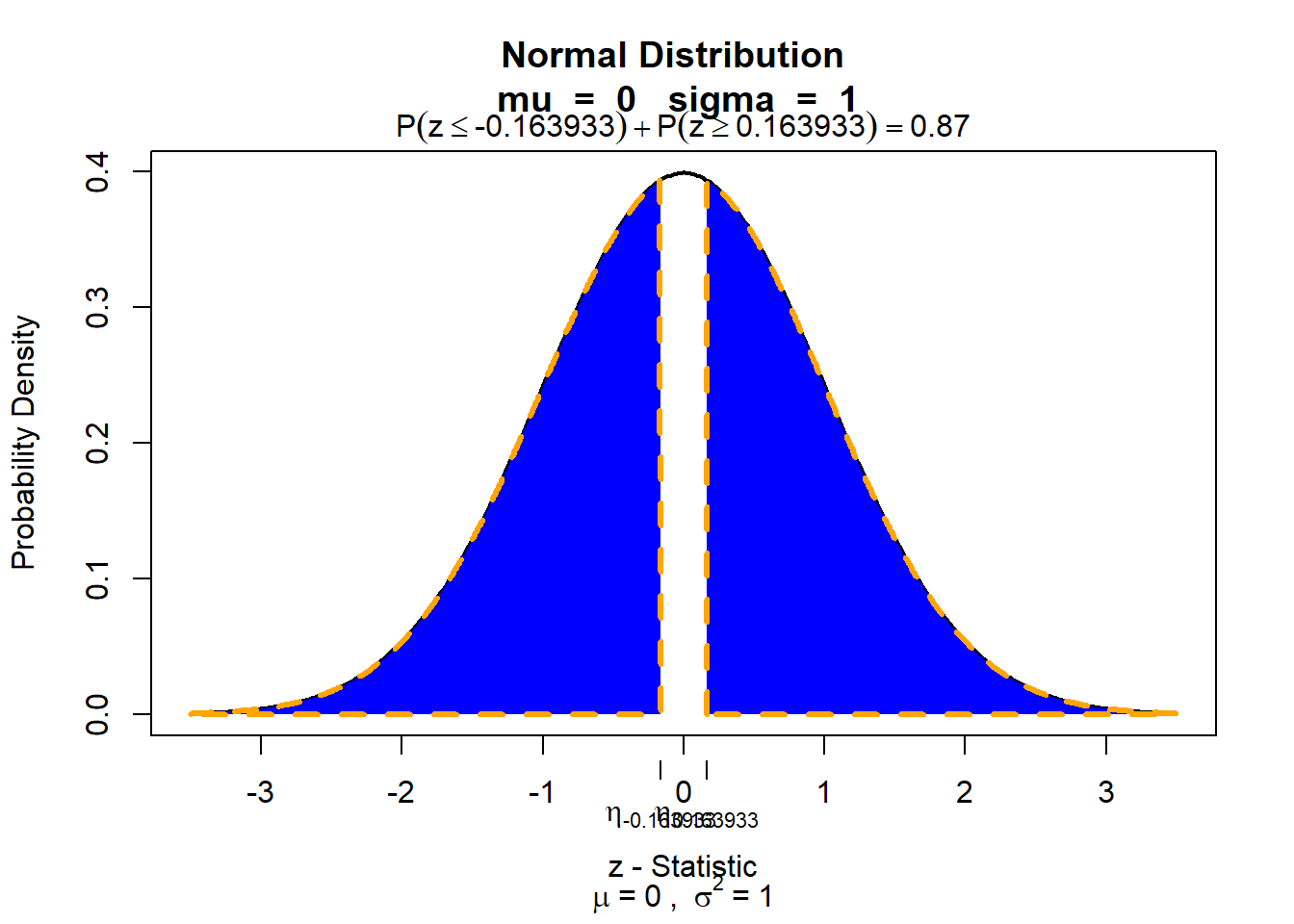
# Define input (change these according to your values)p_hat_1 =500/ (500+44425)p_hat_2 =505/ (505+44405)n_1 =500+44425#this is the total number of subjects in the first groupn_2 =505+44405#this is the total number of subjects in the second groupnull_value =0# Perform calculations (no need to change anything here)p_hat_pooled = (p_hat_1 * n_1 + p_hat_2 * n_2) / (n_1 + n_2)point_est = p_hat_1 - p_hat_2se =sqrt((p_hat_pooled*(1-p_hat_pooled)/n_1)+(p_hat_pooled*(1-p_hat_pooled)/n_2))z = (point_est - null_value)/sepnorm(z)
[1] 0.434892
The lower tail area is 0.4349 (small difference compared to the book due to rounding). The p-value, represented by both tails together, is 0.434892*2 = 0.869784. Because this value \(p > 0.05\), we do not reject the null hypothesis.
Alternatively, we can use the R function prop.test() to test for the difference between the two groups. We used this function in week 4 already for the calculation of a single proportion. The function prop.test is part of the package stats, which is one of the few packages that R automatically loads when it starts. For our purpose, we use it as follow:
result <-prop.test(x =c(500, 505), n =c(44925, 44910),alternative ="two.sided",correct =FALSE)result
    2-sample test for equality of proportions without continuity correction

data:  c(500, 505) out of c(44925, 44910)
X-squared = 0.026874, df = 1, p-value = 0.8698
alternative hypothesis: two.sided
95 percent confidence interval:
 -0.001490590  0.001260488
sample estimates:
    prop 1     prop 2
0.01112966 0.01124471
prop.test(
This is the function that conducts a test for a proportion.
x = c(500, 505),
Here we indicate the number of cases that are in our two groups. In this example, 500 patients who received a mammogram and died and 505 patients who did not receive a mammogram and died. Because these are two values, we combine them using ‘c()’.
n = c(44925, 44910),
The second value specified should be the total number of trials. In our case: the total number of patients in the two groups. Because these are two values, we combine them using ‘c()’.
alternative = "two.sided"
Determine whether we want to use a two sided-test, or a one-sided test. Options are “two.sided” (default), “less” (when \(H_1: \mu < p\)) or “greater” (when \(H_1: \mu > p\)).
correct = FALSE)
With this, we indicate that we do not want to calculate the confidence interval using a ‘continuity correction’. By default, this value is set to ‘TRUE’.
12.3.2.3 Data in a data frame
If you have a data frame with a variable that, for each case, represents one of two possible outcomes (in statistical terms “success” and “failure”), we can use prop.test.
prop.test(table(mammogram$treatment, mammogram$breast_cancer_death), alternative ="two.sided",correct =FALSE)
    2-sample test for equality of proportions without continuity correction

data:  table(mammogram$treatment, mammogram$breast_cancer_death)
X-squared = 0.026874, df = 1, p-value = 0.8698
alternative hypothesis: two.sided
95 percent confidence interval:
 -0.001490590  0.001260488
sample estimates:
    prop 1     prop 2
0.01112966 0.01124471
This is the function that conducts a test for a proportion. We select the independent variable (mammogram$treatment) and dependent variable (mammogram$breast_cancer_death). Note that the order of the variables matters for the confidence interval: so list the independent first and then the dependent variable.
alternative = "two.sided"
Determine whether we want to use a two sided-test, or a one-sided test. Options are “two.sided” (default), “less” (when \(H_1: \mu < p\)) or “greater” (when \(H_1: \mu > p\)).
correct = FALSE
With this, we indicate that we do not want to calculate the confidence interval using a ‘continuity correction’. By default, this value is set to ‘TRUE’.
The results are identical to the example above that used the summary data.
12.4 Reporting the results from a hypothesis test for the difference in two proportions
# Define input (change these according to your values)p_hat_1 =70/330p_hat_2 =90/470n_1 =330#this is the total number of subjects in the first groupn_2 =470#this is the total number of subjects in the second groupnull_value =0# Perform calculations (no need to change anything here)p_hat_pooled = (p_hat_1 * n_1 + p_hat_2 * n_2) / (n_1 + n_2)point_est = p_hat_1 - p_hat_2se =sqrt((p_hat_pooled*(1-p_hat_pooled)/n_1)+(p_hat_pooled*(1-p_hat_pooled)/n_2))z = (point_est - null_value)/sez
[1] 0.7181896
2*pnorm(q=z, lower.tail=FALSE)
[1] 0.4726404
# Results using prop.testprop.test(x =c(70, 90), n =c(330, 470),alternative ="two.sided",correct =FALSE)
    2-sample test for equality of proportions without continuity correction

data:  c(70, 90) out of c(330, 470)
X-squared = 0.5158, df = 1, p-value = 0.4726
alternative hypothesis: two.sided
95 percent confidence interval:
 -0.03603276  0.07729646
sample estimates:
   prop 1    prop 2
0.2121212 0.1914894
Output explanation
the probability of finding the observed (\(z\) or \(\chi^2\), given the null hypothesis (p-value) is given as follows:
in R, see p-value = 0.009823. Note: If the value is very close to zero, R may use the scientific notation for small numbers (e.g. 2.2e-16 is the scientific notation of 0.00000000000000022). In these cases, write p < 0.001 in your report.
12.4.0.1 Reporting
If you calculate the results by hand and obtain a z-score, then the correct report includes:
A conclusion about the null hypothesis; followed by
Information about the sample percentage and the population percentage.
\(z\) = the value of z.
p = p-value. When working with statistical software, you should report the exact p-value that is displayed.
in R, small values may be displayed using the scientific notation (e.g. 2.2e-16 is the scientific notation of 0.00000000000000022.) This means that the value is very close to zero. R uses this notation automatically for very small numbers. In these cases, write p < 0.001 in your report.
If you calculate the results using prop.test and obtain a \(\chi^2\)-score, then the correct report includes:
A conclusion about the null hypothesis; followed by
Information about the sample percentage and the population percentage.
\(\chi^2\) = the value of chi-square, followed by the degrees of freedom in brackets.
p = p-value. When working with statistical software, you should report the exact p-value that is displayed.
in R, small values may be displayed using the scientific notation (e.g. 2.2e-16 is the scientific notation of 0.00000000000000022.) This means that the value is very close to zero. R uses this notation automatically for very small numbers. In these cases, write p < 0.001 in your report.
Report
✓ There is no statistically significant difference between the percentage of citizens who were somewhat dissatisfied with democracy before the election (21.21%, n = 330) and after the election (19.14%, n = 470), z = 0.72, p = 0.47.
✓ There is no statistically significant difference between the percentage of citizens who were somewhat dissatisfied with democracy before the election (21.21%, n = 330) and after the election (19.14%, n = 470), \(\chi^2\) (1) = 0.51, p = 0.47.
If you really like pipes, you can also use: example_data |> pull(party_choice) |> table() .↩︎
If you would like to calculate the confidence interval for the second category, you can use, for example, relevel to re-order the categories of the first variable:
    1-sample proportions test with continuity correction

data:  table(relevel(example_data$party_choice, ref = "Other party")), null probability 0.5
X-squared = 290.52, df = 1, p-value < 2.2e-16
alternative hypothesis: true p is not equal to 0.5
95 percent confidence interval:
 0.7423954 0.7954986
sample estimates:
   p
0.77
This uses a slightly more complicated formula for calculating the confidence interval (Wilson score interval), also incorporating a ‘continutiy correction’ (which accounts for the fact that we are using a continuous normal distribution to approximate a discrete phenomenon, i.e. the number of successes)↩︎